The Auditory Modeling Toolbox
EXP_BAUMGARTNER2013 - Figures from Baumgartner et al. (2013)
Usage
data = exp_baumgartner2013(flag)
exp_baumgartner2013(flags) reproduces figures of the book chapter from Baumgartner et al. (2013).
Optional fields of output data structure:
- data.id
- listener ID
- data.u
- listener-specific uncertainty
- data.dtfs
- matrix containing DTFs. Dimensions: time, position, channel (more details see doc: HRTF format)
- data.fs
- sampling rate of impulse responses
- data.pos
- source-position matrix referring to 2nd dimension of hM and formated acc. to meta.pos (ARI format). 6th col is the lateral angle. 7th col is the polar angle.
- data.spdtfs
- DTFs of specific SPs
- data.polangs
- polar angles corresponding to data.spdtfs
- data.pmv
- predicted polar angular response PMVs
- data.respangs
- polar response angules corresponding to data.p
- data.pe
- predicted local polar RMS error in degrees
- data.qe
- predicted quadrant error
The following flags can be specified:
| 'plot' | Plot the output of the experiment. This is the default. |
| 'noplot' | Don't plot, only return data. |
| 'fig12' | Reproduce Fig. 12: DTFs of median SP (left ear). Left: NH12. Center: NH58. Right: NH33. Brightness: Spectral magnitude. |
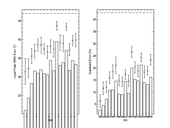
| 'fig13' | Reproduce Fig. 13: Listener's localization performance for non-individualized versus individualized DTFs. Bars: Individualized DTFs. Circles: Non-individualized DTFs averaged over 16 DTF sets. Error bars: ±1 standard deviation of the average. Horizontal line: Chance performance corresponding to guessing the direction of the sound. |
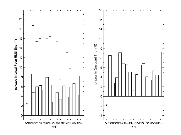
| 'fig14' | Reproduce Fig. 14: Bars: Increase in localization errors when listening to a binaural recording created with the DTFs from NH58. Asterisk: Difference between actual (experiment) and predicted performance when listening to individualized DTFs. Horizontal lines: chance performance corresponding to guessing the direction of the sound. |
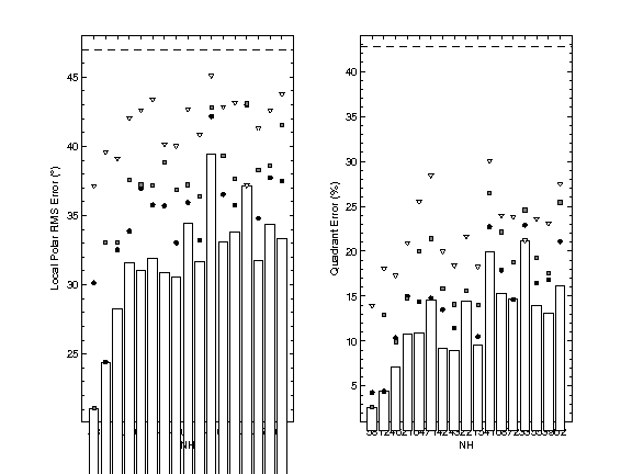
| 'fig15' | Reproduce Fig. 15: Bars: Localization performance of the pool listening to selected DTFs. Circles: DTFs from NH12. Squares: DTFs from NH58. Triangles: DTFs from NH33. |
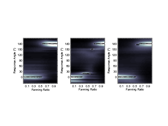
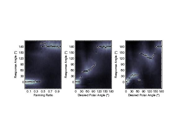
| 'fig18' | Reproduce Fig. 18: Predicted response probabilities (PMVs) as a function of the amplitude panning ratio between a rear and a front loudspeaker in the same SP (lateral angle: 30 deg.). Left: Results for NH12. Center: Results for NH15. Right: Results for our pool of listeners. Circle: Maximum of a PMV. Panning ratio of 0: Only front loudspeaker active. Panning ratio of 1: Only rear loudspeaker active. |
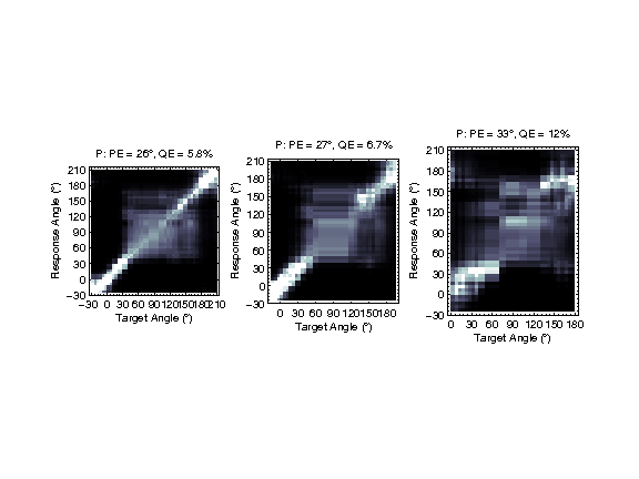
| 'fig19' | Reproduce Fig. 19: Prediction matrices (PMVs) for different loudspeaker spans and NH12. Left: Span of 0 deg. (single-loudspeaker reproduction, baseline). Center: Span of 30 deg. Right: Span of 60 deg. P: Predicted performance. |
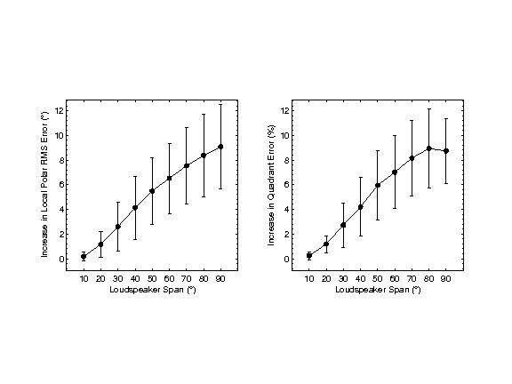
| 'fig20' | Reproduce Fig. 20: Increase in localization errors as a function of the loudspeaker span. Circles: Averages over all listeners from the pool. Error bars: +/- 1 standard deviation of the averages. |
| 'fig22' | Reproduce Fig. 22: Predictions for the surround setups in the VBAP configuration. Left: 5.1 setup, panning between the loudspeakers L and LS. Center: 10.2 setup (DSX), panning from L (polar angle of 0 deg.) via LH2 (55 deg.) to LS (180 deg.) Right: 9.1 setup (Auro-3D), panning from L (0 deg.) via LH1 (34 deg.) and LSH (121 deg.) to LS (180 deg.). Desired polar angle: Continuous scale representing the VBAP across pair-wise contributing loudspeakers. All other conventions as in Fig. 18. |
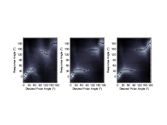
| 'fig23' | Reproduce Fig. 23: Predictions for two modifications to the 9.1 setup (Auro 3D). Left: Original setup, loudspeakers LS and LSH at the azimuth of 110 deg. Center: LSH at the azimuth of 130 deg. Right: LS and LSH at the azimuth of 130 deg. All other conventions as in Fig. 22. |
Requirements:
- SOFA API v0.4.3 or higher from http://sourceforge.net/projects/sofacoustics for Matlab (in e.g. thirdparty/SOFA)
- Data in hrtf/baumgartner2013
Examples:
To display Fig. 12 use
exp_baumgartner2013('fig12');
To display Fig. 13 use
exp_baumgartner2013('fig13');
To display Fig. 14 use
exp_baumgartner2013('fig14');
To display Fig. 15 use
exp_baumgartner2013('fig15');
To display Fig. 18 use
exp_baumgartner2013('fig18');
To display Fig. 19 use
exp_baumgartner2013('fig19');
To display Fig. 20 use
exp_baumgartner2013('fig20');
To display Fig. 22 use
exp_baumgartner2013('fig22');
To display Fig. 23 use
exp_baumgartner2013('fig23');
References:
R. Baumgartner. Modeling sagittal-plane sound localization with the application to subband-encoded head related transfer functions. Master's thesis, University of Music and Performing Arts, Graz, June 2012. [ .pdf ]
R. Baumgartner, P. Majdak, and B. Laback. Assessment of Sagittal-Plane Sound Localization Performance in Spatial-Audio Applications, chapter 4, pages 93-119. Springer-Verlag GmbH, 2013.


